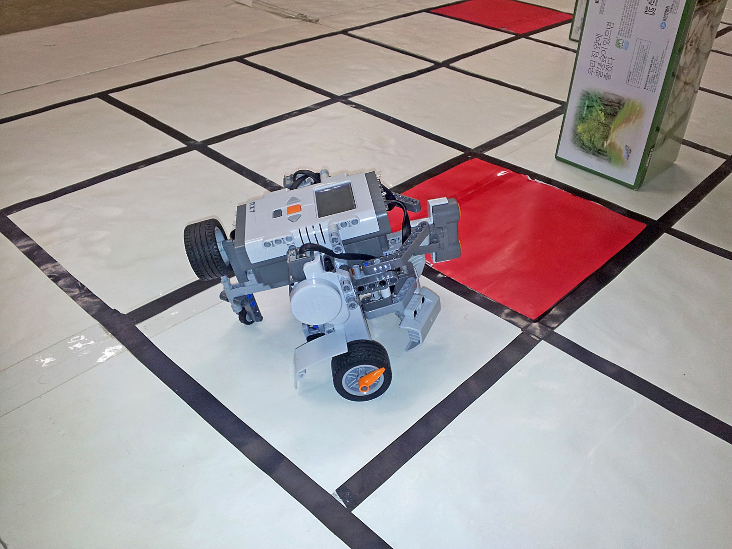
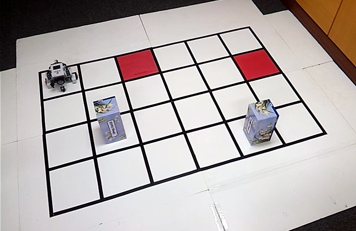
colored cells and obstacles (tissue box).
This robot is designed to explore an environment comprising of a grid of square-shaped cells, whilst avoiding obstacles. Each cell may be colored white or red, which the robot can detect using a color sensor. Obstacles are detected using a forward-facing ultrasonic distance sensor.
The goal is to visit each grid cell and build a map of the world. After determining the state of each grid cell, the robot drives back to the initial starting position.
This page describes the problem and the algorithm that was implemented. There’s a video at the bottom of the page showing the robot in-action.
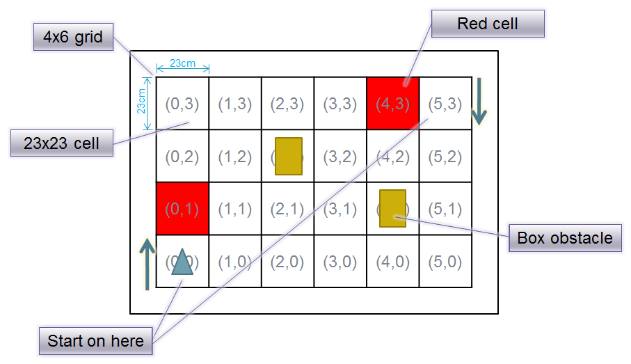
The grid world
The robot’s world is a grid of 4×6 cells, each being a 23 cm square. Each cell can be colored white or red. A cell may also contain an obstacle.
 |
 |
The robot design
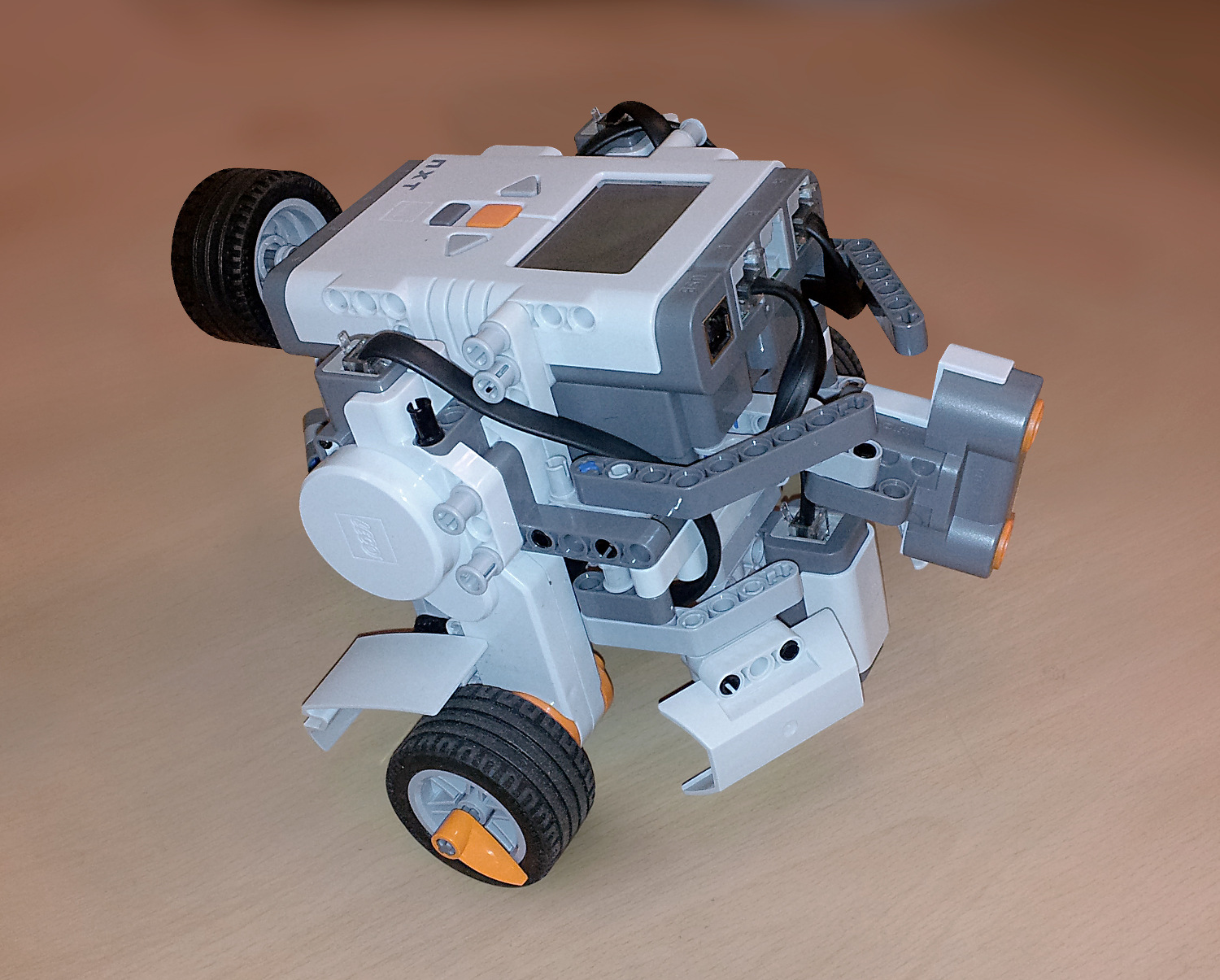
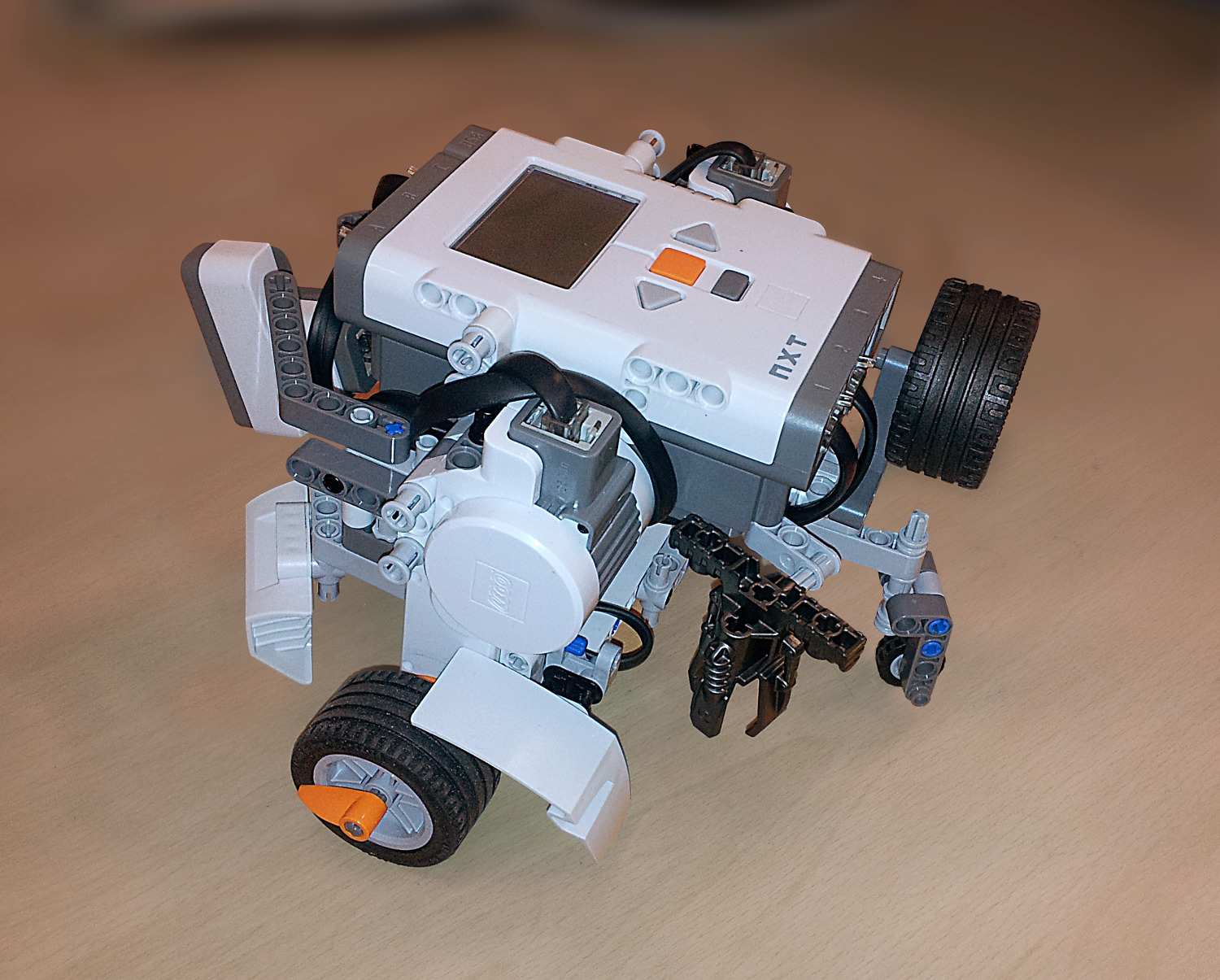
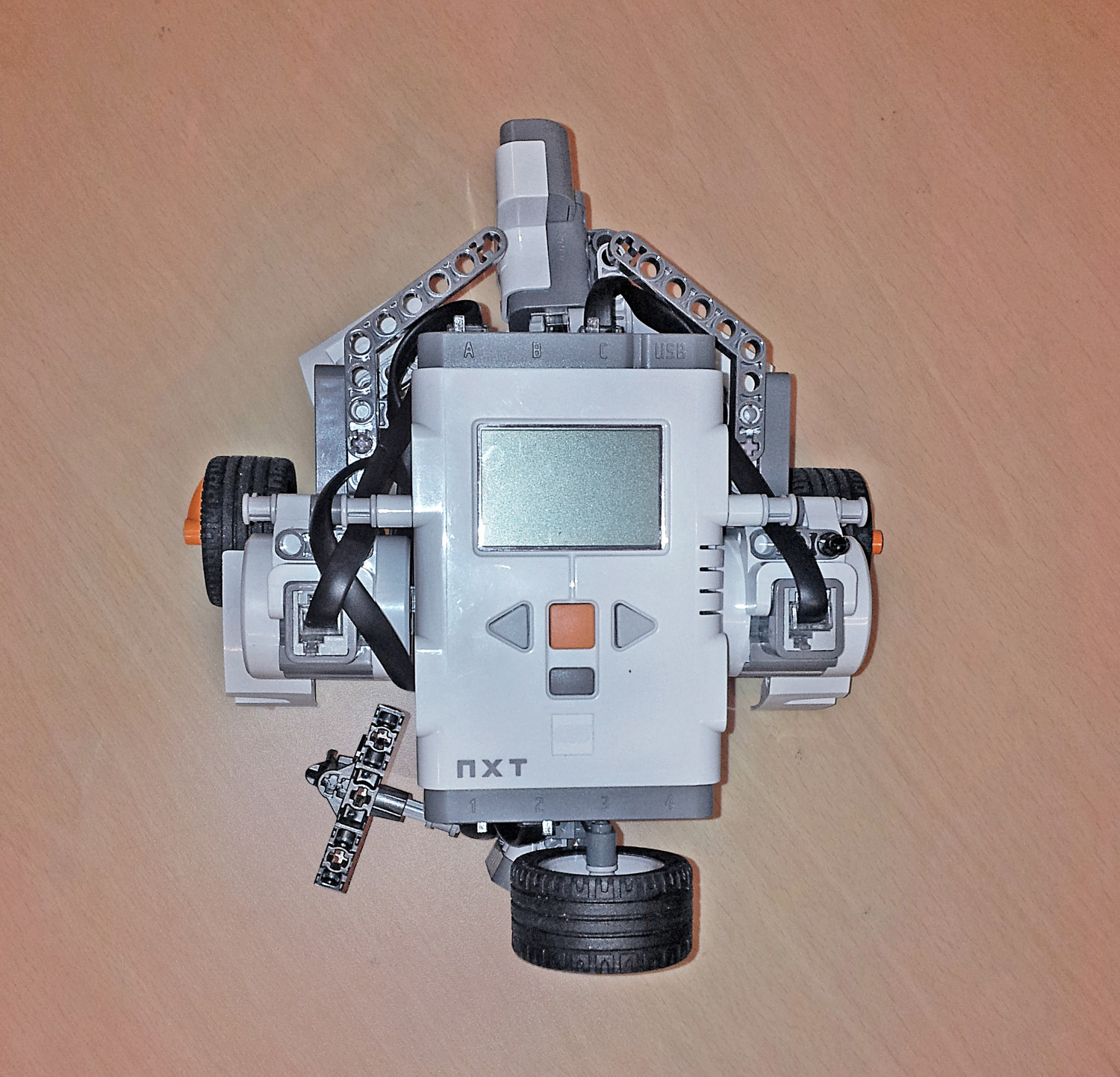
The robot uses two drive motors (differential drive) for simple steering control, with a single pivot wheel (caster) at the back for stability. This design was chosen because it allows the robot to easily rotate in one place, with less wheel-slip than tank treads.
An RGB sensor is used to detect the color of each grid cell (white or red). It is also used to find the line at the edge of each cell, to make sure the robot drives forward exactly perpendicular from the cell boundary. An ultrasonic distance sensor at the front of the robot is used to check for obstacles.
Some of the other parts on the robot are purely cosmetic, like the plastic guards at the front and above the tyres. The objects on the back of the robot, like the spare tyre, provide additional weight above the caster wheel. When the robot decelerates quickly, it’s possible for the robot to tip forward.
 |
 |
 |
Software
The robot was programmed in RobotC. Each behavior is described below:
Driving Forward:
The robot drives forward by a fixed distance of half the cell width. Due to differences between the two motors, there is an accumulation of position error as the robot moves around the map. The robot checks that it is heading in a straight direction by calibrating against each black line that it drives over. Alternatively, a better approach would be to check after 2 or 3 cells, or to use feedback from the wheel encoders.
Turning:
The robot turns on the spot by 90 degrees in each direction, or 180 degrees, by rotating both motors together for a fixed number of encoder ticks.
Checking cell color:
The RGB sensor is used in 7-color mode. Each cell is checked and the color is recorded in the robot’s stored map of the world.
Obstacle detection:
Before the robot moves into the next cell, it checks the distance reading from the ultrasonic rangefinder. If there is a “hit” within 20 cm, an obstacle will be recorded in the robot’s stored map.
Mapping:
The robot records information about the world in an internal map, stored in memory using a 6×8 matrix.
The matrix is initialised with the cell values such that 9 = “out of bounds”, and 0 = “unknown” (Fig. 7, left).
As the robot explores each cell of the grid, the matching row/column in the matrix is updated to reflect the correct state: 1 = “white cell”, 2 = “red cell”, 3 = “obstacle” (Fig. 7, right).
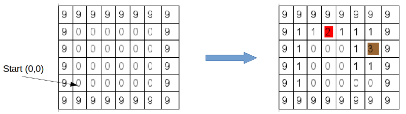 (left) The initial state of the robot’s internal map. (right) Example map state during operation. |
Exploration algorithm:
The robot explores the map in a clockwise direction using a “hug the left wall” algorithm. The basic behaviour is controlled using a FSM (Finite State Machine).
The robot performs the following actions in sequence:
1. Measure current cell color.
2. Check map & determine which cell to move next.
3. Turn towards next cell.
4. Measure distance in-front.
5. Drive forward until just past black line.
6. Turn left, then right, to calibrate forward direction heading.
7. Drive forward to center of next cell.
8. …repeat.
Before moving, the robot checks its map to see which surrounding cells have not been explored. It will move into any cell with a value of “0: unknown”, where the priority order is: left cell first, then forward, then right. If those 3 cells have already been explored, it will turn right if that cell is not an obstacle or out-of-bounds. Otherwise, the robot will turn 180 and go back to the previous cell.
This “hug the left wall” algorithm is repeated for every cell and will allow the robot to successfully navigate most obstacle configurations that were tested. However, if the obstacles are located in adjacent cells, it is possible that the robot will get stuck in one area.
Return-to-start algorithm:
Once the robot has checked each of the 24 cells it plays a tune and returns to the starting cell. First, the robot turns so it’s facing south on the grid, checks its internal map to determine if the cell in front is white or red, then drives forward. Otherwise it turns west and checks that cell, or lastly turns east and checks that direction.
The result is that the robot will drive south for as long as possible, then drive west, while navigating around obstacles. This algorithm results in the shortest path back to the home position, however it could have been made faster by checking the southern and western cells without actually turning the robot to face that direction first.
Performance
The robot successfully maps the grid world and returns to the home position in a total time of approximately 3 minutes, 15 seconds.
 |